Mapping Crystalline Regions During In-Situ Heating- Comparing TEM and 4D STEM
- Abstract number
- 190
- Presentation Form
- Submitted Talk
- Corresponding Email
- [email protected]
- Session
- Stream 2: EMAG - In-situ microscopy
- Authors
- Benjamin Miller (1), Anahita Pakzad (1), Liam Spillane (1), Bernhard Schaffer (1), Cory Czarnik (1)
- Affiliations
-
1. Gatan, Inc.
- Keywords
In-Situ
Python
Real-Time Processing
4D STEM
Crystallization
High Resolution TEM
Nanoparticles
- Abstract text
Often during in-situ TEM experiments, it is important to see and distinguish crystalline regions in a sample. Whether grains in a polycrystalline sample, nanoparticles on an amorphous support, or crystals nucleating from an amorphous material, the ability to detect these crystalline regions is valuable. Yet, this can be challenging for several reasons. In a large TEM image, it may be difficult to see at a glance the extent of crystalline regions because neighboring regions are not easily distinguished, or because the large image cannot be displayed at full resolution on the monitor. When using 4D STEM, it is also inherently difficult to see anything as visualization requires a dimensional reduction that can hide important information. In both cases, the difficulty is increased if a series of images or data cubes are acquired as part of an in-situ experiment.
In this work, we demonstrate Python-based processing of both 4D STEM and high-resolution TEM images to map the spatial distribution of crystalline regions. This can be done (with some limitations) during live during acquisition, or it can be applied to previously acquired datasets. In the case of 4D STEM, each diffraction pattern is processed to find the maximum intensity pixel, while masking a user-defined central region of the pattern. The direction from the pattern center, spacing, and intensity of this maximum point are determined, and color maps are produced. The hue can be either the angle or distance from center while the brightness of the color is determined by the intensity. A 2D color map is thus generated from each 4D data cube. If a series of data cubes is acquired, this results in a color video. This approach can be extended for processing large high resolution TEM images. First a grid of overlapping windows is extracted from a single large 2D image, and the FFT of each window is computed. These FFTs are placed into a 4D cube which is analogous to that generated using 4D STEM, but with diffractograms instead of diffraction patterns. This 4D cube of FFTs can then be analyzed in the same way as a 4D STEM data cube.
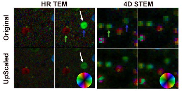
This processing approach has been applied to repeated in-situ melting and crystallization of Sn nanoparticles. During acquisition, it was not obvious that the nanoparticles recrystallize in different orientations each time, but this is clear from the processed data. It also becomes obvious from the processed HR TEM video that some particles crystallize before others, as seen in Figure 1. It is not possible to see this in the 4D STEM data, due to the temporal resolution we achieved with that technique (one 24x24 pattern data cube every ~10 s).
Figure 1. Maps generated from 2 consecutive frames from 2 in-situ series of HR TEM images and 4D STEM datasets of the same cluster of particles. For both types of data, a similar mapping technique has been applied. The 2nd row of maps shows spatially upscaled data (upscaled by a factor of 2). Blue and green arrows indicate where the same 2 particles appear in all the maps. White arrows indicate a particle (green in the map) which crystallized <0.5 s later than 2 other particles (blue and red). This was detectable due to the good temporal resolution of the in-situ TEM technique.
While we are processing the 4D STEM data and the HR TEM data in a similar way, there are differences and tradeoffs which make each technique optimal for some different experiments. The primary benefit of the HR TEM technique is the ability to capture data with the excellent temporal resolution afforded by TEM and modern in-situ cameras. In the data we will present, images were captured at 20 fps, but much higher framerates are possible. However, the spatial resolution of the FFT-based maps tends to be poor. This is because a large number of pixels in the TEM image must be processed to generate a single map pixel. In the data shown in Figure 1, a 128x128 region in the image generates a single map pixel. This can be mitigated to some extent by overlapping the analysis windows (in this case, we process a new 128x128 region every 32x32 pixels), but this oversampling results in some blurring or delocalization in the maps, and the spatial resolution of the technique becomes less well-defined. Finally, the volume of reciprocal space that is sampled using HR TEM is small when compared to 4D STEM. This means that for the same sample region, more lattice spacings will be observed using 4D STEM. This is especially pronounced for TEMs without aberration correction, and many crystalline regions will be missed in any given analysis simply because they are not in a suitable orientation, and thus no lattice spacings are visible1.
For both 4D STEM and the FFT-based processing of HR TEM images, the resulting maps tend to have few pixels. This can be partially mitigated by upscaling the pixel size of the maps as shown in Figure 1, similarly to work by researchers at Oxford2. To do this properly, some other dimension in the data must be summed. For the 4D STEM case, this can be in the diffraction patterns, and for the HR TEM case, it can be the temporal dimension.
Ultimately, the goal for this processing is to perform it live during acquisition to guide decision making at the microscope. The processing speed is a limiting factor at the moment, with one 1728x1728 pixel frame processed into a 55x55 pixel map every 3 seconds. However, with better parallelization of the processing in Python, faster CPUs or GPUs, and other optimizations, this will undoubtedly become faster in the future. Processing 4D STEM data cubes is already fast in comparison, since computationally expensive FFTs are not required. As long as data does not need to be pre-processed (e.g. to remove outliers) a similar 55x55 pixel map can be produced in just 0.5 seconds, so the 4D STEM technique is limited by the acquisition, not data processing.
- References
1. Fraundorf, P., Qin, W., Moeck, P. & Mandell, E. Making sense of nanocrystal lattice fringes. Journal of Applied Physics (2005).
2. Jones, L. et al. Managing dose-, damage-and data-rates in multi-frame spectrum-imaging. Microscopy (2018).